Droplet based microfluidics
In this second part of the tutorial, the basic process for setting up an automatic control is shown, manually first and with our tools after. It is assumed that you are familiarized with all the basic operating of your system and that you have correctly set up the SDK environment as it was shown in the first chapter of the tutorial. If you didn’t see it before, please, go for it first.
The purpose of this Jupyter Notebook is to work as a quick guide to the SDK development with the Elveflow products. The process shown using a OB1 Pressure Controller with a FS5D Flow Sensor, but it works also for any other Elvesys product.
Also, before starting with this introduction, make sure you have read all the documentation related to your purchased products. Disregarding that information could increase the risk of damage to the equipment, or the risk of personal injuries. In case you don’t have a copy, you can download all the documents from our website.
The content of this chapter of the tutorial is the following:
This tutorial has been written and tested using Windows 10, 64bits, Python 3.8.8, Jupyter Notebook 6.3.0 in October, 2021. The pressure controller is an OB1 MK3+ and the flow sensor a FS5D.
The PI Controller or Proportional-Integrative Controller is a basic linear controller, yet powerful for lot of situations, which makes the output of the controlled system to follow a desired curve of values, called reference, and ensures that the system properly works and that it is stable for the operating expected situation.
To achieve this control of the system’s output, it takes the current system’s output value, calculates the difference to the reference (the desired output), which is called error, and makes some operations with it.
The operations for a basic PI Control are two: the proportional term calculus and the integrative term calculus.
Note. Usually, the integrative gain is expressed as integrative time which is related to the integrative gain through the sampling period of the controlling system, but it is shown here this way as may be considered more understandable with gains.
The PI code is only a translation of the previous equations to the Python language:
error = p_sens - p_ref i_error += error P_val = K_P * error I_val = K_I * i_error p_control = P_val + I_val
In the next code cell you can run the initialization of the system. After it, you will find the place where you can put your controller code inside the main execution routine that was shown in the previous chapter of this tutorial.
Before running the following code, change all the paths, OB1 values and sensor values to match your system.
# INITIALIZATION # Tested with Python 3.5.1 (IDE Eclipse V4.5.2 + Pydev V5.0.0) # Add python_xx and python_xx/DLL to the project path # coding: utf8 import sys from email.header import UTF8 sys.path.append('C:/dev/SDK/DLL64/DLL64') # Add the path of the library here sys.path.append('C:/dev/SDK/Python_64') # Add the path of the LoadElveflow.py from ctypes import * from array import array from Elveflow64 import * import time import matplotlib.pyplot as plt # # Initialization of OB1 ( ! ! ! REMEMBER TO USE .encode('ascii') ! ! ! ) # Instr_ID=c_int32() print("Instrument name and regulator types are hardcoded in the Python script") # See User Guide to determine regulator types and NIMAX to determine the instrument name error=OB1_Initialization('01BECD3F'.encode('ascii'),3,2,0,0,byref(Instr_ID)) # All functions will return error codes to help you to debug your code, for further information refer to User Guide print('error:%d' % error) print("OB1 ID: %d" % Instr_ID.value) # Add one digital flow sensor with water calibration (OB1 MK3+ only), all information to declare sensors # are described in the User Guide error=OB1_Add_Sens(Instr_ID, 2, 4, 1, 0, 7, 0) # (CustomSens_Voltage_5_to_25 only works with CustomSensors and OB1 from 2020 and after) print('error add digit flow sensor:%d' % error) Calib=(c_double*1000)() # Always define array this way, calibration should have 1000 elements while True: answer=input('Select calibration type (default, load, new ) : ') Calib_path='C:\\Users\\Public\\Desktop\\Calibration\\Calib.txt' if answer=='default': error=Elveflow_Calibration_Default (byref(Calib),1000) break if answer=='load': error=Elveflow_Calibration_Load (Calib_path.encode('ascii'), byref(Calib), 1000) break if answer=='new': OB1_Calib (Instr_ID.value, Calib, 1000) error=Elveflow_Calibration_Save(Calib_path.encode('ascii'), byref(Calib), 1000) print ('calib saved in %s' % Calib_path.encode('ascii')) break else: print("Not recognized command.") if error==0: print("Done.")
Instrument name and regulator types are hardcoded in the Python script error:-301706 OB1 ID: -1 error add digit flow sensor:-8003 Select calibration type (default, load, new ) : default Done.
The code for controlling the system would be something like the following code if you do it with a custom controller. You have first two functions which run the control over the system and, after that, you can find a code in which you can change the values of the parameters of the controller.
If your microfluidic circuit is not very hydraulically resistive, you may need to add some flow resistance to it in order to make use of the whole ranges of your flow sensor and pressure regulators.
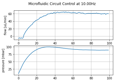
Remember that each microfluidic system needs a different PI Controller tuning, thus, the results you will have may be different to the ones obtained with my testing setup. Try the proposed parameters values or change those values if you are confident, but avoid to make huge changes on the parameters at a time to maintain the system within safety limits.
period = 0.1 # 10Hz p_error = 0 i_error = 0 meas_flow = c_double() def pid_run(): global p_error global i_error start_t = time.time() # <- This must be close to the routine last_t = start_t # Main routine while True: # Get the current output error=OB1_Get_Sens_Data(Instr_ID.value, fs_channel, 1, byref(meas_flow)) flow_list.append(meas_flow.value) # Calculate the mathematical error p_error = ref_flow - meas_flow.value i_error += p_error # PI Controller equations P_val = K_p * p_error I_val = K_i * i_error # Anti-windup I_val = max(I_min, min(I_max, I_val)) # Final control action p_control = P_val + I_val p_control = max(p_min, min(p_max, p_control)) # Safety saturation error_list.append(p_error) control_list.append(p_control) p_control=c_double( float(p_control) ) # Convert to c_double error=OB1_Set_Press(Instr_ID.value, p_channel, p_control, byref(Calib), 1000) # Return error message # Check if the elapsed time match the time limit if (time.time() - start_t) > experiment_t: break # Wait until desired period time sleep_t = period - (time.time() - last_t) if sleep_t > 0: time.sleep( sleep_t ) last_t = time.time() # And update the last time # Turn off the pressure p_control = 0.0 error=OB1_Set_Press(Instr_ID.value, p_channel, p_control, byref(Calib), 1000) # Return error message def plot(): # Plot the signals plt.rcParams['axes.grid'] = True fig=plt.figure() fig.suptitle("Microfluidic Circuit Control at {0:.2f}Hz".format(1/period)) plt.subplot(2,1,1) plt.plot( flow_list ) plt.ylabel('flow [uL/min]') plt.subplot(2,1,2) plt.plot( control_list ) plt.ylabel('pressure [mbar]') def run(): pid_run() plot()
Change the following values to tune the controller for your system. You can also change the reference value and the experiment execution time by some values more useful for your application. If the system follows your reference too slowly, you may increase the proportional and/or the integrative gain. If it is too aggressive, the contrary. Feel free to play with them by changing the values in small steps.
Also check that the control maximum and minimum values are good for your system.
# Controller parameters: Very soft controller K_p = 0.05 # <- Change this value to tune the controller K_i = 0.1 # <- Change this value too to tune the controller ref_flow = 60 # uL/min p_min = 0 # <- This is only negative if you have some vacuum source p_max = 1000 # <- This depends on the Z regulator of each channel # OB1 arrangement p_channel = 2 # <- Change this to fs_channel = 2 # <- your real configuration experiment_t = 10.0 # Seconds flow_list = [] error_list = [] control_list = [] run()
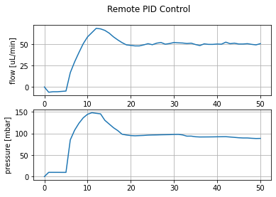
If you have previously configured any of the compatible instruments (OB1, AF1, MSRD, BFS) in remote mode, where the acquisition is run autonomously, the Elvesys SDK allows you to start or stop PID loops between these instruments without having to write the code of the loop itself. A fully working flow regulation can be started with an OB1 and an MFS with a single function call. Subsequent modification of the PID target is achieved in the remote loop of the device controlling the pressure/flow. A PID loop can be started on a single remote loop if the device can regulate the pressure/flow and a sensor is also connected to it.
The following is a summary of the necessary functions to run the remote PID controller:
If you correctly tuned the controller in the previous step of this chapter, you should now have a set of parameters which is suitable for your current system. You can set those values in the next code cell to run the remote PI controller with them. Anyway, notice that the sampling frequency of the remote PID control is higher than the achievable with custom external code; thus, you may need to reduce the value of your gains.
Note. If you need to check the usage of one function from our SDK, you can find the API reference at the SDK User Guide at any moment.
In [4]:
# Controller parameters: Very soft controller K_p = 0.05 # <- Change this value to tune the controller K_i = 0.003 # <- Change this value too to tune the controller ref_flow = 50 # uL/min experiment_t = 5.0 # OB1 arrangement p_channel = 2 # <- Change this to fs_channel = 2 # <- your real configuration # Start running the PI Control on remote mode error = OB1_Start_Remote_Measurement(Instr_ID.value, byref(Calib), 1000) # Start the PID Controller onsite p_channel = c_int32( int(p_channel) ) # convert to c_int32 fs_channel = c_int32( int(fs_channel) ) # convert to c_int32 error = PID_Add_Remote(Instr_ID.value, p_channel, Instr_ID.value, fs_channel, K_p, K_i, 1) # Set the reference ref_flow = c_double( float(ref_flow) ) error = OB1_Set_Remote_Target(Instr_ID.value, p_channel, ref_flow) flow_list = [] control_list = [] meas_flow = c_double() control_val = c_double() start_t = time.time() # <- This must be close to the routine last_t = start_t while True: error = OB1_Get_Remote_Data(Instr_ID.value, fs_channel, byref(control_val), byref(meas_flow)) flow_list.append( meas_flow.value ) control_list.append( control_val.value ) # Check if the elapsed time match the time limit if (time.time() - start_t) > experiment_t: break # Wait until desired period time sleep_t = period - (time.time() - last_t) if sleep_t > 0: time.sleep( sleep_t ) last_t = time.time() # And update the last time error = OB1_Stop_Remote_Measurement(Instr_ID.value) print('Stop. Error value: %d' % error) # Plot the signals plt.rcParams['axes.grid'] = True fig=plt.figure() fig.suptitle("Remote PID Control") plt.subplot(2,1,1) plt.plot( flow_list ) plt.ylabel('flow [uL/min]') plt.subplot(2,1,2) plt.plot( control_list ) plt.ylabel('pressure [mbar]')
Stop. Error value: 1
Out[4]:
Text(0, 0.5, 'pressure [mbar]')
In this tutorial we have seen how a simple PI Control works, how can it be implemented with the OB1 instrument, how to tune its parameters and, finally, how to use the remote PID controller.
As we saw, it is not difficult to implement a custom controller for the OB1 instrument using Python. However, the problem gets more difficult when you must perform more tasks while running the controller or if you must control several instruments at once. For those situations, it turns out way easier to use the remote PID controllers due to the fact that, once configured and launched, you only must change the reference or gather data from it whenever you need it.
Although in this tutorial the PI controllers have been tuned using the Python code, you can also use the ESI for that purpose if it is more comfortable for you as the values must be the same. But if you are going to use a custom controller, remember to check that the sampling frequency matches the one of the control you used for the tuning.
Finally, if you want to keep learning about microfluidics and related topics, you can also check our application notes (free tutorials) or reviews.
Hope you found this tutorial useful, and thanks for trusting Elvesys!
How can we help you?
Name*
Email*
Message
Newsletter subscription
We will answer within 24 hours
By filling in your info you accept that we use your data.
Do you want tips on how to best set up your microfluidic experiment? Do you need inspiration or a different angle to take on your specific problem? Well, we probably have an application note just for you, feel free to check them out!
Microfluidics is the science of handling small amounts of liquids, inside micrometer scale channels. Discover how to handle fluids for your microfluidic experiments.
This application note demonstrates a smart use ouf Elveflow's Pressure sensor and sensor reader for Direct-Ink-Writing flow control.
Learn how to set up your development environment for Elveflow products with this comprehensive tutorial.
This user guide will show you how to run microfluidic colocalization studies of single molecule spectroscopy.
This application note explores the basic principle of pneumatic pumps and a flow controller based on the basic principle of pneumatic pumps, known as pressure driven flow control. It also demonstrates the applications of pressure driven flow control in a range of industrial & research fields.
Flow regulation is a compulsory operation in most of the microfluidics operations. In some applications such as 2D or 3D cell culture, flow regulation is essential since accurate micro-environmental parameters control is required. Elveflow do it’s best to make this operation as easy as possible to help you to focus on what really matter in your setup.
Study the impact of molecular transport on cell cultures with a cross flow membrane chip and microfluidic instruments.
Precise liquid injection system for manipulation of small volumes of fluids using the MUX distribution and the MUX recirculation valve.
This application note explains how to set up a robust and reproducible microfluidic platform for liposomes assembly with improved encapsulation efficiency and reduced polydispersity in size.
Single-wall carbon nanotubes (SWCNTs) are considered as quasi 1-dimensional (1D) carbon nanostructures, which are known for their outstanding anisotropic electronic, mechanical, thermal and optical properties.
This application note describes how to combine and synchronise liquid perfusion and imaging using an Olympus spinning disc confocal microscope together with an Elveflow pressure-driven flow controlled microfluidic system.
Mixing is a crucial step for several microfluidic applications like chemical synthesis, clinical diagnostics, sequencing and synthesis of nucleic acids
This application note describes how microfluidic can be employed as a nanoparticle generator based on the example of PLGA bead generation.
Learn how to perform PLGA nanoparticle preparation with Elveflow instruments and a microfluidic chip
The application note describes how to convert various units of shear stress and/or pressure from one to another: shear stress conversion from Pascal, atmosphere, and N/m²...!
Get a quote
Collaborations
Need customer support?
Serial Number of your product
Support Type AdviceHardware SupportSoftware Support
Subject*
I hereby agree that Elveflow uses my personal data Newsletter subscription
Message I hereby agree that Elveflow uses my personal data Newsletter subscription