Flow Control for Toxicity Testing and Exposure
Steady, repeatable flow for a defined toxicant exposure, from a dose gradient to a whole-organism test.A dose gradient in one run, steps ~10 ms to setpoint.
Same dose every run, no pipetting scatter.
A gas or aerosol, dosed at the air–liquid interface.
A commercial chip, your device, or a whole organism.
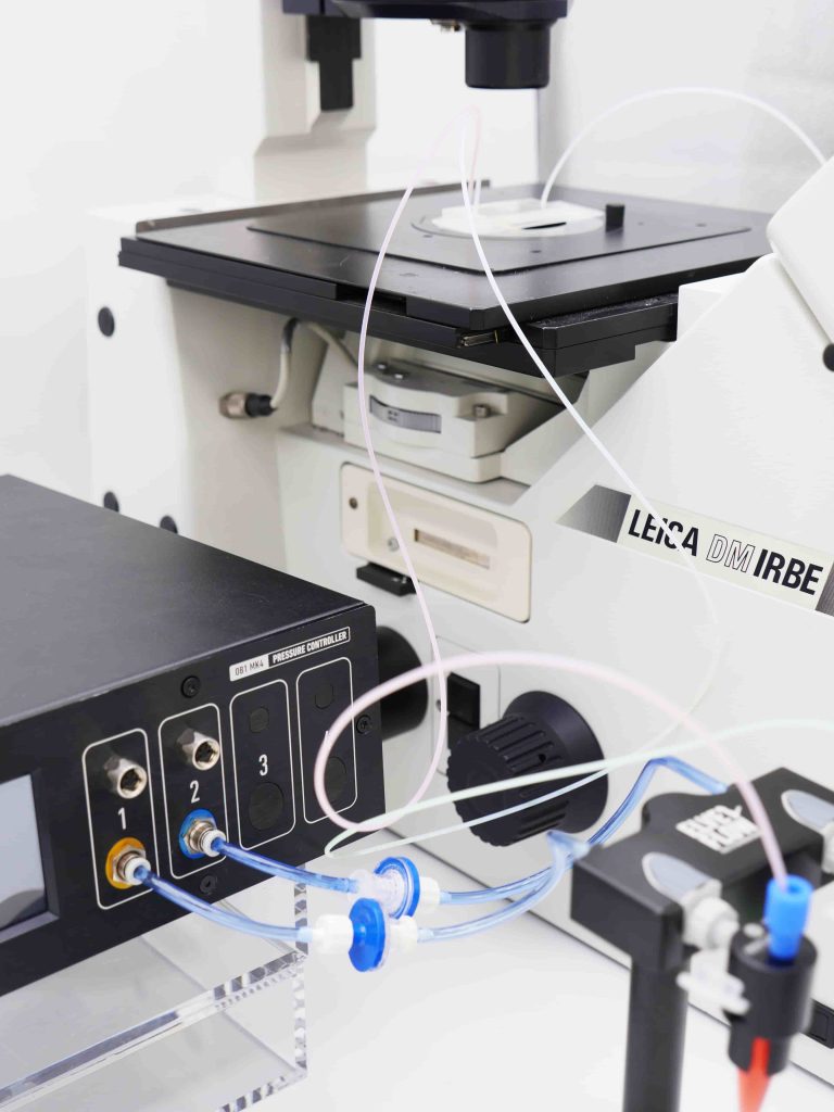
A cell or tissue model meets a defined toxicant dose when pressure-driven flow control delivers it, in liquid at a set flow rate from 0.1 µL/min to 500 mL/min or as a graded gas across an air–liquid interface.
-

Dr. Hayden Taylor
University of California, Berkeley, United States
We are using the device extensively at the moment and I have been quite impressed by its capabilities -

Dr. Arne Lüken
Chemical Process Engineering at RWTH Aachen
The Elveflow OB1 enables us precise pressure and flow control and measurement in various microfluidic and lab scale projects from tissue engineering to membrane filtration analysis. -

Dr. Nelson BC Serre & Dr. Matyáš Fendrych
Cell Growth Lab, Department of Experimental Plant Biology, Charles University, Czech Republic
After an easy installation, we are now using the OB1 and flow sensors routinely and are very satisfied by both the flow stability and the software user-friendly interface. -

Seongjin Park, Senior Engineer
Department of Physics, Syracuse University
We use Elveflow instrument in several projects and they are great to work with. The LabVIEW implementation was also very successful. I hope more people can get to know the OB1 system -

Dr. Pushparani Micheal Raj
Max Planck Institute of Quantum Optics, MAX IV Laboratory
I have extensively used Elveflow systems in the world's most brilliant X-ray source. Elveflow systems are precise, controlled and adaptive to many samples under adverse conditions.
Features & Benefits
Pressure-driven flow control for toxicity testing
A toxicity result is only as good as the exposure behind it. In a static well, a dose goes in all at once. It spikes, the cells take it up, and it breaks down, so the concentration the model meets drifts away from the dose you meant to test. Hand-pipetted dilution series add their own scatter between replicates. Under flow you control the exposure directly. You deliver a set concentration and hold it, step to the next, or run it for days. The exposure becomes the variable you test, not a source of noise. Two things then decide whether flow suits a toxicity assay: how stable and controlled it is, and how well it fits the model and the readout. Syringe and peristaltic pumps are the usual starting point, and a rocker plate is common too. Each has a weak point here.
Syringe pump. A motor advances a plunger at a set speed, so you dial in a flow rate directly, which is why it is the usual first pump for dosing. Two limits show up in a toxicity assay. At the low flow rate a long exposure needs, the delivery turns pulsatile, moving in small steps that shear-sensitive cells feel. And the syringe holds a fixed volume, so it stops to refill partway through a run: a wash-in, a washout, or a timed step to the next concentration breaks at that moment, and the dose reaching the cells is uneven. Reopening the line to reload risks a bubble or a contamination the assay can’t afford.
Peristaltic pump. For a repeated-dose or chronic exposure it earns its place, because it recirculates: it returns a costly test solution to its reservoir for reuse across a run of several days. The cost is pulsation. The rollers squeeze the tubing in turn, so the flow pulses with each one, and the pulsation grows with the flow rate. A clean dose-response reads that pulsation as noise, and a shear-sensitive model feels it. Over a long run the repeated squeezing also wears the tubing: the walls stop springing back the same way, so the volume moved per turn changes and the calibrated flow rate drifts, carrying the exposure you meant to hold with it.
Rocker plate. A rocker or gravity plate needs no pump at all: it tips the plate back and forth, and the medium runs to the low side on each tilt. The flow is a by-product of that motion. It reverses direction every cycle, rises and falls within each rock, and the only handles are the tilt angle and the rocking interval. So the concentration and the shear a cell meets swing through the cycle, hard to set to a target dose or to reproduce from one run to the next.
Pressure controller. A pressure controller acts on the solution from the gas side, with no moving part in the liquid, so the flow is continuous from the first second and carries no pulse, up to 20× steadier than a syringe or peristaltic pump. It reaches the setpoint in about ten milliseconds, so a change in concentration lands as a clean step and the level holds steady between changes. It never touches your toxicant or your medium, so it adds no contamination of its own. That stability and speed hold at every scale, from a single exposure chamber to a gradient across a whole chip.
Deliver the dose your model actually sees
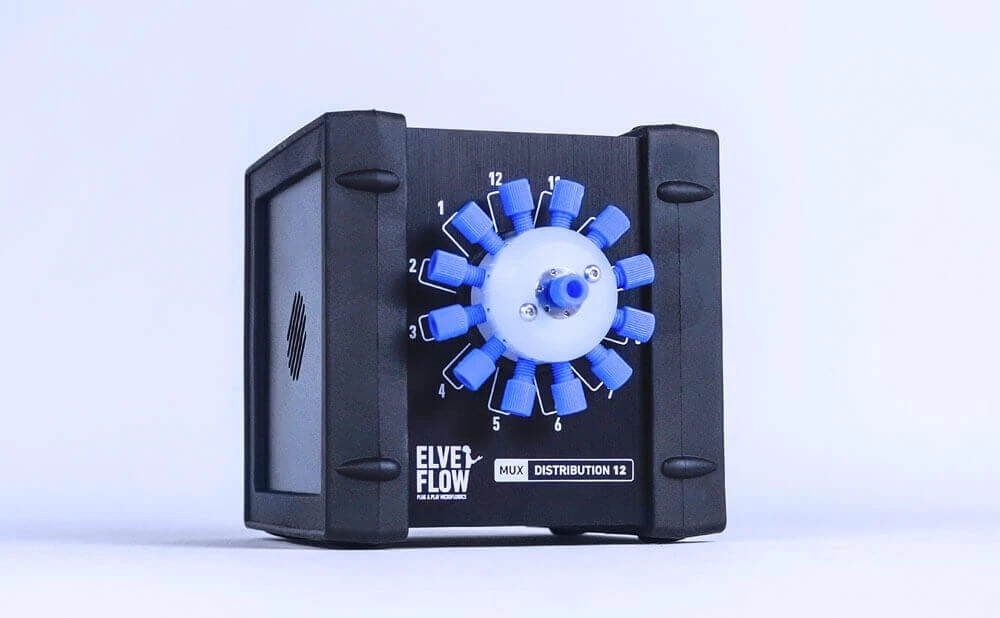
Two tools shape the concentration your model meets. A gradient-generator chip splits one stock into a row of concentrations at once. Pressure-driven flow control drives its inlets at the flow rates that fix each step, so one run gives a full concentration-effect curve, every dose in parallel. A distribution valve handles the timing. It routes a dose, then a rinse, then the next dose down the same line, on the sequence you program, so a repeated challenge or a washout runs without reconnecting tubing. Between switches the concentration holds steady. And each switch settles fast, so the model sees a square change, not a slow smear. The dose is defined in both strength and timing.
Expose to a gas or an aerosol
Not every toxicant reaches cells in liquid. An airborne pollutant, a vapour, an inhaled drug, or an aerosol meets the airway as a gas, at an air–liquid interface. Pressure-driven flow control reaches that too, because it delivers vacuum as well as pressure. Draw air and a test gas through a gradient generator with a steady negative pressure, and you build a gas concentration gradient across the chip, the same way you would in liquid. The airway model then meets a defined, graded dose of what it would actually breathe. The lung-chip study below used exactly this to expose bronchial cells to a formaldehyde gradient and read the damage down the dose.
Run a repeated-dose or chronic exposure
Some toxicity shows up only after days of exposure, not minutes. The setup then has to keep going without someone at the bench. Pressure draws medium from a reservoir of any size, a millilitre or several litres, at the same rate whichever you use. A larger reservoir simply extends the run. A recirculation loop returns the test solution to its reservoir, so a costly compound serves the whole multi-day exposure and is not wasted. A repeated-dose or chronic study runs over days or weeks, and a stable exposure that runs on its own is what makes it practical. You program the exposure once, and it runs.
Automate an exposure and follow the endpoint
A toxicity timeline can run long, and every step has to land on time: a dose held for a set window, a rinse, a second dose, a readout at fixed points. You lay that timeline out once in the software, and it runs on its own, through the night and across days if the study needs it. TTL lines (0/5 V) tie the dosing to the instruments around it. They can trigger a microscope to capture a frame at a set moment, or advance a stage through a row of conditions, so every image carries a known dose and time. Put a detector downstream, and the steady flow carries whatever the cells shed, an enzyme or a stress marker, out to it in real time. The readout is then time-resolved across the whole exposure. For custom automation, use the SDK in Python, MATLAB, LabVIEW or C++.
Reproducible exposure for animal-free methods
For a toxicity method, reproducibility is essential. A regulatory agency or a validation body accepts a New Approach Methodology only when it gives the same answer in another lab’s hands. The exposure is one place variation creeps in. Hand-pipetted doses, a flow that drifts as tubing warms, a medium change an hour late: each shifts the concentration-time profile the cells experience, and with it the endpoint. Fixing the delivery removes that source. With a flow sensor closing the loop on the set flow rate, the same programmed exposure plays out identically from one operator, one day, one site to the next. What differs between runs is then the biology under test, not the dosing. That is what lets a result travel, and it lines up with where regulatory agencies are heading: the FDA Modernization Act and its roadmap to reduce animal testing, and parallel moves on industrial chemicals and cosmetics.
Application
Inhalation toxicity in a lung chip
An airborne toxicant reaches the lung as a gas, at an air–liquid interface. Pressure-driven flow control can draw that gas across a chip as a defined gradient. Chen and colleagues built a modular lung chip to find out how formaldehyde, a common indoor pollutant, damages human bronchial epithelial cells across a range of concentrations [Frontiers in Bioengineering and Biotechnology, 2025, 1]. They drew air and formaldehyde through the chip’s gradient generator with our pressure controller, running in vacuum. A steady negative pressure pulled the two gas streams through and built a rising formaldehyde gradient across four parallel lines of cells. Cell viability fell line by line as the dose rose, and oxidative stress climbed with both dose and time. RNA sequencing traced the damage to ferroptosis and flagged twelve ferroptosis-related genes. Adding the ferroptosis inhibitor deferoxamine restored viability and lowered the reactive oxygen species, which pinned formaldehyde’s toxicity on that pathway.
Aquatic and developmental toxicity in a fish-embryo test
Some safety questions are about a whole organism and its environment, not a cell line. Panuška and colleagues built a 3D-printed millifluidic chip to run the Fish Embryo Test on zebrafish under continuous perfusion, and to measure the toxicity of a model teratogen [RSC Advances, 2021, 2]. They perfused the embryos’ medium and delivered the toxicant with our pressure controller and a flow sensor, holding the flow across the full 96-hour test. Flow ran at 80 µL/min for an hour to load, then at 30 µL/min for the run, while an automatic routine imaged each embryo every fifteen minutes. The embryos developed normally under perfusion. The test scored both the median lethal dose and the teratogenic malformations. It read a stronger toxic effect from ethanol than the standard multiwell assay does, in line with the OECD Fish Embryo Acute Toxicity guideline (TG 236).
Liver-function monitoring in a fatty-liver model
Hepatotoxicity often shows up first as a drop in what the liver makes. A readout that follows a hepatocyte-function marker while the cells are challenged is a useful safety signal. Lopez-Muñoz and colleagues built a label-free plasmonic biosensor to follow albumin from a fatty-liver model, continuously and without a label [Nanomaterials, 2020, 3]. Albumin is a protein hepatocytes secrete and a marker of liver function. They drove the sample stream past the biosensor at a constant flow with our pressure controller, so the albumin signal stayed steady and comparable across the run. The sensor tracked albumin down to the picomolar range, and it told the fatty-liver model from its control by how much albumin it secreted. The authors put the readout forward for studying the disease and for hepatotoxicity assessment.
[1] Chen S, Li Z, Yan Q, Hua C, Shang P, Liu K, Zhao J, Jin G, Li X, Xie F. Development and application of a stepwise-assembled modular biomimetic lung chip for analyzing formaldehyde-induced cellular ferroptosis. Frontiers in Bioengineering and Biotechnology. 2025;13:1570270. doi:10.3389/fbioe.2025.1570270
[2] Panuška P, Nejedlá Z, Smejkal J, Aubrecht P, Liegertová M, Štofik M, Havlica J, Malý J. A millifluidic chip for cultivation of fish embryos and toxicity testing fabricated by 3D printing technology. RSC Advances. 2021;11(33). doi:10.1039/d1ra00846c
[3] Lopez-Muñoz GA, Ortega MA, Ferret-Miñana A, De Chiara F, Ramón-Azcón J. Direct and Label-Free Monitoring of Albumin in 2D Fatty Liver Disease Model Using Plasmonic Nanogratings. Nanomaterials. 2020;10(12):2520. doi:10.3390/nano10122520
| OB1 MK4 | |||||
|---|---|---|---|---|---|
| PNEUMATIC SPECIFICATION | |||||
| Channel pressure range | 0 to 200 mbar(1) (0 to 2.9 psi) |
0 to 2,000 mbar(1) (0 to 29 psi) |
0 to 8,000 mbar(1) (0 to 116 psi) |
-900 to 1,000 mbar(1) (-13 to 14.5 psi) |
-900 to 6,000 mbar(1) (-13 to 87 psi) |
| Pressure stability(2) | 0.015 % FS(1) 0 µbar (0.0004 psi) |
0.005 % FS(1) 100 µbar (0.0014 psi) |
0.006 % FS(1) 500 µbar (0.007 psi) |
-900 to 500 mbar | -900 to 2,000 mbar |
| 0.005 % FS(1) 100 µbar (0.0014 psi) |
0.005 % FS(1) 350 µbar (0.005 psi) |
||||
| 500 to 1,000 mbar | 2,000 to 6,000 mbar | ||||
| 0.007 % FS(1) 150 µbar (0.0021 psi) |
0.007 % FS(1) 525 µbar (0.0076 psi) |
||||
| Response time(3) | Down to 10 ms | ||||
| Setting time(4) | Down to 50 ms | ||||
| Minimum pressure increment | 0.006 % FS(1) 12 µbar (0.00017psi) |
0.006 % FS(1) 120 µbar (0.0017 psi) |
0.006 % FS(1) 480 µbar (0.007 psi) |
0.0064 % FS(1) 120 µbar (0.0017 psi) |
0.0064 % FS(1) 420 µbar (0.006 psi) |
| Pressure supply | 1.5 bar (or Max pressure + 0.5 bar) to 10 bar Non corrosive, non explosive, dry and oil-free gases, e.g. air, argon, N2, CO2, … |
||||
| Input vacuum(5) | / / |
Any value from -0.7 to -1 bar Compatible with vacuum pump or vacuum line |
|||
| Input pneumatic connector | 6 mm push-in | ||||
| Output pneumatic connector | 4 mm push-in | ||||
| Liquid compatibility | Non contact pump Any aqueous, oil, or biological sample solution. |
||||
| FLOW CONTROL | |||||
| Flow sensor compatibility | Compatible with the whole MFS and BFS range Monitoring and feedback loop flow control available | ||||
| Flow sensor compatibility | From 0,1 µL/min to 500 mL/min (indicative, please refer to the MFS and BFS series) | ||||
| Flow sensor compatibility | Non-contact pump Any aqueous, oil, or biological sample solution. | ||||
| CONTROL & MONITORING | |||||
| Software control | Elveflow Smart Interface – Windows 10, 11, both 32 and 64 bit versions supported | ||||
| Software Development Kit | Libraries available: Matlab, Python, LabView, C++ | ||||
| Flow sensor compatibility | Non-contact pump Any aqueous, oil, or biological sample solution. – Windows 10, 11, both 32 & 64 bit versions supported Serial/UART communication protocol on request | ||||
| Data management | Possibility to log and extract data (CSV), channel and sensor detailed information using ESI | ||||
| Input profiles | Possibility to load profiles: ramp, sine, triangle, square, or custom | ||||
| Automation | Generate step-by-step sequences using the ESI built-in sequence management Log and export custom configurations (CSV) | ||||
| Screen | LCD screen showing pressure and sensor flow rate in real time | ||||
| ELECTRICAL SPECIFICATIONS | |||||
| Voltage | 24V | ||||
| Typical power | 12W | ||||
| Power connection | DC power connector, Plug, 3A, 2.1mm, 12mm | ||||
| Interface | USB Type B | ||||
| Communication type | Serial | ||||
| Sensor connection | M8 4-pins, one connector per channel | ||||
| Compatibilit | Elveflow sensors: MFS, BFS, MPS, MFP, MBD Custom sensors: 5 to 24V supply voltage, 0 to 10V readout voltage | ||||
| Triggers | Input and Output TTL signal 0V or 5V | ||||
| Supply Voltage Range (V) | 100 to 240 VAC | ||||
| Supply AC Frequency (Hz) | 50 to 60 Hz | ||||
| Maximum Output Current (A) | 1.67 A | ||||
| Maximum Output Power (W) | 40 W | ||||
| MECHANICAL SPECIFICATIONS | |||||
| Dimensions (length x width x height) | 240 x 223 x 83 mm | ||||
| Weight | 1.4 kg to 2.9 kg | ||||
(1) Max pressure value might vary by +/- 2.5% (2) Pressure stability (standard deviation) measured over the full pressure range with an external high accuracy pressure sensor (Druck DPI150) (3) Time required to reach 5% of the setting point. Depending on your computer’s operating system (4) Time required to reach 95% of the set point. Volume dependent – Measurement was done on 12 mL reservoir for a set point from 0 to 200 mbar (5) A vacuum source is mandatory for calibration and use of dual channels even if the channels are to be used in pressure only.
Frequently Asked Questions
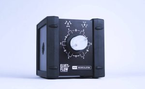
The Elveflow OB1 is a pressure controller that governs how a toxicant reaches your model and for how long. It pushes a liquid dose from a sealed reservoir at a flow rate you set, pulseless and responding in about ten milliseconds. Paired with an Elveflow flow sensor, it holds that flow rate through the run. With an Elveflow MUX distribution valve, it steps between solutions in sequence: a dose, a wash, then the next dose. And because it also delivers vacuum, it can draw a gas or an aerosol across an air–liquid-interface chip. It does not supply the model or the readout; it controls the exposure. So a cell monolayer, a 3D model, an organ-on-chip, or a whole-organism device meets a defined, repeatable dose you can defend as a New Approach Methodology.
For toxicity work, the deciding factor is whether the dose stays exactly what you set, run after run. Pressure-driven control is the option that does. A syringe pump turns pulsatile at the low flow rates a long exposure uses and pauses to refill, which interrupts a wash-in or wash-out and pushes the dose around. A peristaltic pump will recirculate a compound over a long study, but its rollers add a pulse whose size tracks the flow rate. A rocker moves medium by tilting the plate, so the dose and the shear follow the rocking cycle, not a value you dial in. The Elveflow OB1 delivers continuous flow from a non-contact pressure source, reaches its setpoint in roughly ten milliseconds, and runs up to four independent lines at once. You can expose several conditions side by side and read them against each other in one experiment. Because the pressure acts on the gas above the reservoir, the instrument never contacts your toxicant.
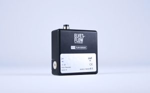
Think of the exposure in two parts, the concentration and the timing, and the Elveflow OB1 governs both through the flow. The concentration is set by your solutions, and for a whole range at once, by a gradient-generator chip. The OB1 drives that chip’s inlets, and an Elveflow MFS or BFS flow sensor holds each inlet flow rate in a feedback loop, so the concentrations the chip lays down stay fixed through the run. The timing is set by an Elveflow MUX distribution valve. It steps one line through a dose, a wash, then the next dose, up to twelve solutions in a programmed order, and several valves chain together past twelve. So the numbers on your dosing plan come from the chemistry you prepare, and the OB1 makes sure the model receives them, at the concentration and on the timing you specified.
Yes, and doing it on a chip is faster and tighter than a plate of hand-made dilutions. Pair the Elveflow OB1 with a gradient-generator chip. The OB1 drives the chip’s inlets at held flow rates, the chip mixes one stock into a graded row of concentrations, and every chamber sees its dose at the same moment under the same flow. That is the advantage for a concentration-effect curve: every point is acquired in parallel, from the same starting material. The differences you measure come from the dose, not from pipetting scatter or timing gaps between wells. Read viability, a stress marker, or whatever endpoint your assay reports across the row, and the curve falls out of one experiment.
Yes. Gas-phase exposure uses the vacuum side of the instrument. Because the Elveflow OB1 delivers vacuum as well as pressure, it can draw a test gas through a gradient generator and across an air–liquid-interface chip. This builds a gas concentration gradient over the cells. In one lung-chip study, an OB1 held a steady negative pressure that pulled air and formaldehyde through the chip and generated the formaldehyde gradient the bronchial cells met. Viability fell and oxidative stress rose down that gradient [Frontiers in Bioengineering and Biotechnology, 2025, 1]. So inhalation and respiratory-toxicity work, on a vapour or an aerosol, is within reach on the same instrument.
Yes. The Elveflow OB1 draws from reservoirs holding a millilitre to several litres, so a long perfusion has the volume to run for days without a refill. You program the exposure sequence once, and it proceeds on its own overnight and across days. For a repeated-dose or chronic study, an Elveflow MUX recirculation valve can return the medium to its reservoir, so a costly test compound serves the whole run and is not wasted. A non-contact design keeps the pump out of the fluid path, and the programmed profile handles each dose and wash. A multi-day exposure runs without stop-start handling at the bench.
Yes. The Elveflow OB1 controls the exposure regardless of what the substance is: a drug or its metabolite, an industrial or agricultural chemical, a cosmetic ingredient, an airborne pollutant, or a nanomaterial in suspension. It drives any aqueous or biological solution through your chip or model at a set, repeatable flow rate. Its vacuum mode covers gas-phase and air–liquid-interface exposure for airborne agents. That breadth is why the same instrument serves next-generation risk assessment across pharmaceuticals, chemicals, cosmetics and the environment. It fits wherever a defined, animal-free exposure has to stand up.
Yes. A whole-organism test like the zebrafish Fish Embryo Test runs under continuous perfusion when the Elveflow OB1 supplies the flow. In one study, an OB1 with an Elveflow flow sensor perfused zebrafish embryos for the full 96-hour test and delivered the toxicant, holding the flow while the embryos developed and an automatic routine imaged each one. The perfused test scored the median lethal dose and teratogenic endpoints, and it read a stronger toxic effect than the standard multiwell assay [RSC Advances, 2021, 2]. It maps onto the OECD Fish Embryo Acute Toxicity guideline (TG 236), so it fits aquatic ecotoxicology and developmental-toxicity screening.
The Elveflow OB1 keeps the flow steady so a real-time readout stays quantitative; the readout itself comes from your assay. Place an inline sensor or assay downstream of the model. A steady flow lets you follow what the cells release, an enzyme, a secreted marker, or a stress signal, as the exposure runs, with no discrete sampling. In a fatty-liver study, an OB1 held a constant flow that carried the sample past a label-free biosensor tracking albumin, a liver-function marker [Nanomaterials, 2020, 3]. For viability or oxidative-stress endpoints read by imaging, a TTL trigger lines the OB1’s flow up with image acquisition, so dose and image share one clock. The OB1 controls the flow; you choose the endpoint and the assay.
Yes, and for toxicity that reproducibility is the whole point. With an Elveflow MFS or BFS sensor holding the flow in a feedback loop, the Elveflow OB1 replays the same dose on the same timing every run, whoever is at the bench. The dosing stops being one of the things that shifts between replicates or between labs. That transferability is exactly what a validation body checks before it accepts a New Approach Methodology. A method that gives a different answer in another lab’s hands is not one a regulatory agency can rely on. It is timely, too. The FDA Modernization Act and its roadmap to reduce animal testing, alongside parallel moves on chemicals and cosmetics, are pushing toxicology toward standardised, animal-free data. A delivery you can reproduce helps a result meet that bar.
Yes. The OB1 is chip- and model-agnostic. It pushes solution into any reservoir and through standard tubing, so it drives a commercial toxicity chip, your own PDMS device, a biosensor chip, or a millifluidic device holding whole organisms, all the same way, with any aqueous or biological solution. If your setup is unusual, tell us the model and your target flow rate, and we will confirm the configuration. Whatever exposure format your assay needs, the OB1 fits it.
The Elveflow OB1 is a non-contact pump, so the instrument never touches your toxicant or your medium. The fluid path is only the reservoir, tubing and vessel, which means fewer parts to prepare and one less route for contamination across a long exposure. The reservoirs, caps and tubing Elveflow supplies are autoclavable. You sterilise them before each run and prepare the wetted path as you would for any sterile assay. No sterility certification is claimed for the instrument itself, since it stays outside the fluid path.
Yes. Once you have entered the dosing timeline and any solution switches into the Elveflow Smart Interface, the Elveflow OB1 carries it out on its own. An overnight or multi-day exposure needs no one at the bench. Its TTL lines (0/5 V) hand timing back and forth with your other instruments. The OB1 can trigger a microscope to grab an image at a set point, take a trigger from the microscope to launch a dose, or pace a fraction collector to sample the outflow at fixed intervals. For tighter integration, the SDK drives it from Python, MATLAB, LabVIEW or C++. The flow record streams to CSV as the run goes, so the dose history is there when you analyse the endpoint.
Contact us through the form and tell us your assay, the chip or model you use, and the exposure profile you need, liquid or gas, single-dose or chronic. We will help you match the OB1 configuration, sensors and accessories to your toxicity workflow, and answer setup questions before you buy.

 Job
Job Collaborations
 Customer
 Other
Other