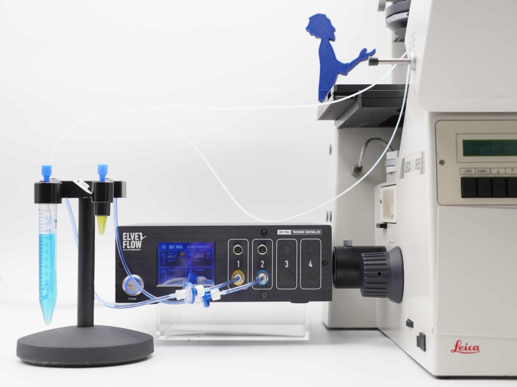
Flow Control for Gels AND Biomaterials
Every phase on its own pressure, held while the material forms.Switching time sets the segment length.
Stop-flow cycles on a defined pressure difference.
One sequence, from the first drop to the last.
0.005% of full scale, flow held with a sensor.
Fibre diameter, particle size and printed geometry follow the flow that forms them. Our pressure controller sets the pressure behind it, to 0.005% of full scale, or holds a set flow rate with a sensor in the line.

-

Dr. Hayden Taylor
University of California, Berkeley, United States
We are using the device extensively at the moment and I have been quite impressed by its capabilities -

Dr. Arne Lüken
Chemical Process Engineering at RWTH Aachen
The Elveflow OB1 enables us precise pressure and flow control and measurement in various microfluidic and lab scale projects from tissue engineering to membrane filtration analysis. -

Dr. Nelson BC Serre & Dr. Matyáš Fendrych
Cell Growth Lab, Department of Experimental Plant Biology, Charles University, Czech Republic
After an easy installation, we are now using the OB1 and flow sensors routinely and are very satisfied by both the flow stability and the software user-friendly interface. -

Seongjin Park, Senior Engineer
Department of Physics, Syracuse University
We use Elveflow instrument in several projects and they are great to work with. The LabVIEW implementation was also very successful. I hope more people can get to know the OB1 system -

Dr. Pushparani Micheal Raj
Max Planck Institute of Quantum Optics, MAX IV Laboratory
I have extensively used Elveflow systems in the world's most brilliant X-ray source. Elveflow systems are precise, controlled and adaptive to many samples under adverse conditions.
Features & Benefits
Pressure-driven flow control for structured soft materials
The geometry you report is set at the nozzle. A fibre’s segment length, a bead’s diameter, a capsule’s wall thickness, a thread’s composition sequence: each one follows the flow at the moment the material forms, and that flow follows the pressure drop across the circuit, Q = ΔP/R. What makes this work harder than most flow work is that R does not stay put. A precursor gels, a solution thickens, a nozzle narrows, so the resistance climbs while the run is going and the flow moves with it. Some of the polydispersity you publish belongs to your driving hardware.
Batch methods. Bulk emulsification under a stirrer, or dripping by hand from a needle into a crosslinker bath, is the baseline this field measures itself against. For a first formulation screen it is also the fastest route on the bench. Nothing in it is a setting. Size and spread come out of the process, so there is no setting to record, sweep, or hand to the next person, and a reviewer asking for the same batch twice is asking for something the method cannot give.
Volumetric displacement, bought or built. A motor advances a plunger at a commanded speed, so the flow rate is imposed kinematically, and viscosity does not shift it in steady state. No gas line to plumb. It is the default for extrusion printing and for most droplet work, and open-source versions of it circulate. Three costs land on this kind of work. The stepping is not silent. In ordinary operation it puts a fluctuation of one to two percent on the flow, at a frequency that climbs with the flow rate. In your geometry it arrives as a percent-level swing in diameter along the object. You set the plunger speed, so the pressure at the nozzle is whatever the circuit demands, with no direct handle on it as a precursor thickens. A gelling line then announces itself as a thickening filament or a popped fitting, instead of a number you could have acted on. And each new speed has to charge the compliance of the tubing before it shows up at the nozzle, which is dead time in the middle of a print, with a refill interruption once the barrel empties.
Pressure-driven control. Gas above the liquid does the pushing, so nothing mechanical moves in your precursor, and the driving pressure carries no periodic component of its own. Two things can make that pressure, and they mark your object differently. A solenoid regulator works by switching. It overshoots on the way to a new setpoint, and keeps a small oscillation once it gets there. That overshoot is printed into the first stretch after every ink change, so a segment shorter than the transient never reaches the value you asked for. In droplet work it pushes the junction briefly into another regime, and the first drops after each change come out of family. The oscillation writes itself along the object as a periodic variation in diameter, which widens your size histogram and reads as chemistry. A piezoelectric valve moves continuously to the setpoint and holds it there, with no switching cycle in the loop. Ours is piezoelectric, and it holds to 0.005% of full scale, so the spread you report comes from your chemistry and your chip.
Sweep in fine steps, and stop where it works
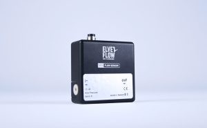
You enter a pressure, or a flow rate with an MFS or BFS sensor in the line. Either way the instrument delivers a pressure, and Q = ΔP/R turns it into flow through your circuit. Two figures then decide how far you can go, and how finely you can place the value. The range of the module you pick fixes the ceiling. Ours run from 200 mbar for a low-resistance nozzle up to 8 bar for a narrow one or a viscous precursor, with vacuum ranges for pulling instead of pushing. Our minimum increment is 0.006% of full scale, which is 120 µbar on a 2 bar module, so a sweep across a formation regime runs as a list of setpoints you enter once. Because the actuator acts on the gas above the liquid, it adds no dead volume to your line and touches none of your precursor.
Hold the flow when the resistance climbs
Pressure control imposes a pressure difference. It does not, on its own, impose a flow rate. Pair the controller with an MFS or BFS flow sensor and the loop closes. The sensor measures the flow, the controller moves the pressure until the measured flow matches the value you asked for, and it keeps moving as the circuit changes. That matters here more than in most applications, because R drifts for reasons that are part of the protocol. A precursor crosslinks in the line. A gel-forming solution thickens on its way to the nozzle. A nozzle partly narrows. Viscosity also follows temperature, which stays your control in your setup. Without a sensor in the line the pressure setpoint stays defined, and the flow follows the resistance. Say which of the two you are holding, and the numbers in your methods section stay honest.
Switch inks inside a continuous print
Our controller responds in about 10 ms. That is the pressure at the controller. The flow at your nozzle then settles through the resistance and compliance of your tubing and chip, which is the part you can shorten by using stiffer, narrower tubing. Alternating two ink lines turns that speed into structure: composition changes along the extruded object instead of between objects, and the switching time sets the segment length. Profiles come as steps, ramps, sines, triangles, squares, or a curve you upload, so a graded transition between two compositions is entered once and repeated.
Hold a ratio, and adjust each phase independently
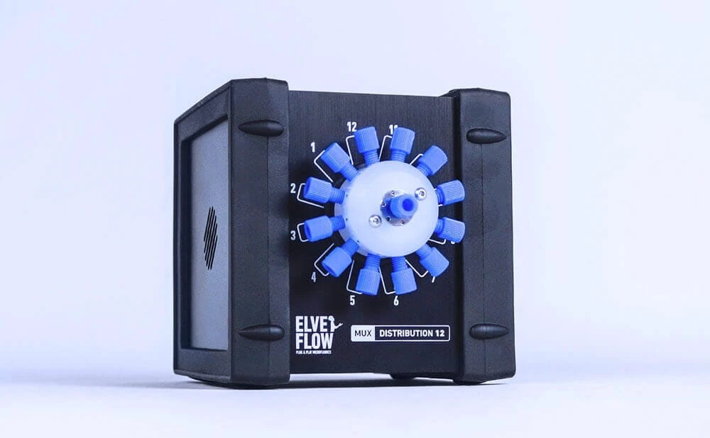
Each channel carries its own setpoint, and a ratio needs exactly that: an oil phase against an aqueous one at a flow-focusing junction, a core against a shell in a coaxial nozzle, or three formulations arriving in a fixed proportion. When one composition thickens faster than the others, giving it its own line lets you raise only that pressure and leave the rest of the geometry alone. A MUX distribution valve puts several precursors on one line and one nozzle, the arrangement a formulation screen needs. Each candidate runs through the same chip, the same nozzle and the same setpoint, with nothing taken apart in between, so a difference in the object you get is a difference in the chemistry. Your channels stay free for the phases that need a pressure of their own. And the same channels drive a gas phase as readily as a liquid one, which is how the bubble size in a foamed precursor gets set.
Hold the formation regime that sets the drop size
A gel formed inside a drop takes its geometry from a balance at the junction: the dispersed phase against the continuous one, at a given viscosity and interfacial tension. Two things decide what comes out. The ratio between the two lines, and how steadily each one holds. Put each phase on its own line and that ratio becomes a pair of setpoints you can write down, sweep, and come back to next month. Drift on either line moves that pair, and a pair that moves widens the size distribution you end up reporting. Changing size is the same operation, a new pair of setpoints, so a series of diameters comes out of one run on one chip. The same balance carries a core against a shell in a coaxial junction, a third phase for a double emulsion, and several aqueous inlets for a microgel built with separate compartments. Solidification stays on your side, whether that is an ionic bath, a temperature change, a light source, or a solvent leaving the drop.
Automate the run, and log what it did
A sequence built once in the Elveflow Smart Interface runs the pressure programme on its own, stage by stage: a hold, a step to a new setpoint, a ramp, a sine, or a profile you upload. A long print goes through without anyone at the panel, and the same file runs again next week. Pressure and flow stream to CSV as it goes, so every object carries the numbers that made it. Triggers in and out tie the sequence to your printer and your camera, and the SDKs drive it from Python, MATLAB, LabVIEW or C++ when the pressure has to follow a path computed elsewhere.
Reproduce the same conditions next month
Fabrication scatter is mostly setup scatter. When what drives the flow is a number you enter, a sequence you can replay and a log you keep, the same file reproduces the same setpoints in another operator’s hands and on another day. Only the material and the chip are left to differ between runs, the two things you wanted to study. Someone else can repeat it too: a value published with its range and its stability is something they can enter on their own instrument.
Application
Hydrogel optical fibre, segment length
The composition of the extruded material can change along its length, without stopping the print. Kafrashian and colleagues set out to make a soft optical fibre that emits light along its length, which calls for a guiding material and a scattering material to alternate along the fibre [Advanced Materials, 2025, 1]. Barrel adapters from our pressure controller were fitted to the two ink syringes, and the pressure was alternated between the two channels, with switching times from 0.5 to 15 s tested across the work. Both inks were diacrylated Pluronic F-127, a physical gel in the syringe at the authors’ processing temperature of 22.7 ± 0.6 °C, printed through a Y-shaped nozzle with two 0.5 mm inlets and a 1 mm outlet. Our controller held the pressure on each ink line; the study measured the segment length and position along the fibre, and the side-emission profile that followed. Segments came out below 500 µm in one continuous process, with their length set by the switching time, in fibres 1 mm across whose emission profile was designed along their length.
Multi-material hydrogel thread, composition sequence
The ratio between two precursors needs lines that move independently. Tillinger and colleagues wanted to print soft multi-material structures without inks contaminating each other, by assembling a thread from separate aqueous droplets held apart by phospholipid bilayers in an oil stream [Small Methods, 2026, 2]. Four channels of our pressure controller drove the reservoirs, one for the oil and one for each of the three hydrogel compositions, with the third held higher because its viscosity rose over time. Our controller held the pressure at each reservoir; the study measured the droplet sequence along the thread and the resolution of the printed pattern. The threads carried droplets 465 ± 15 µm across, deposited into Hilbert-curve patterns and cured into stable structures, with each material staying in its own compartment along the printed path.
Stop-flow lithography patch, crosslinking degree
Here the pressure difference is part of the patterning step itself. Steinbeck and colleagues wanted hydrogel sheets carrying two different crosslinking degrees, and so two porosities, within one micron-scale structure [Small, 2025, 3]. UV light shaped by a transparency mask polymerised the precursor inside a microfluidic channel, in stop-flow mode. Our pressure controller set the pressure difference that moved each finished patch out of the exposure window between shots, and later compressed the patches at a defined pressure difference for mechanical characterisation. The material systems were PEGDA with GMA as comonomer and PNIPAM crosslinked with BIS, patterned through circular mask spots 40 µm across, with highly crosslinked regions from 7 to 52 µm in diameter. Our controller held the pressure difference; the study measured the crosslinking degrees inside each patch and how the pattern changed the compression behaviour. At least two crosslinking degrees were obtained within a single patch, and the printed pattern decided how that patch compressed.
Temperature-responsive microcapsule, shell and gap
A layered capsule wall takes three phases, each on its own setpoint. Kim and colleagues wanted a temperature-responsive capsule that holds a hydrophilic payload in its core, separated from the shell by a gap [Advanced Functional Materials, 2020, 4]. A supersaturated monomer solution was left to separate into a monomer-poor and a monomer-rich aqueous phase. Our pressure controller then drove all three phases into a chip as inner, middle and outer fluid, and the double emulsions were cured under UV. Our controller held the pressure on each of the three lines; the study measured the core-gap-shell architecture that resulted and its use for temperature-triggered biomolecular sensing. A single step delivered the gap as the drops formed, with no later assembly stage, and the capsules held a hydrophilic payload inside the core.
[1] Kafrashian Z, Brück S, Rogin P, Khamdan M, Farrukh HSUB, Pearson S, del Campo A. Segmented, Side-Emitting Hydrogel Optical Fibers for Multimaterial Extrusion Printing. Advanced Materials. 2025;37(4):2309166. doi:10.1002/adma.202309166
[2] Tillinger D, Armendarez NX, Najem JS. Multi-Material Droplet-Based Hydrogel Threads for Extrusion 3D Printing. Small Methods. 2026;10(5):e00928. doi:10.1002/smtd.202500928
[3] Steinbeck L, Paul R, Litke J, Karkoszka I, Wiese GP, Linkhorst J, De Laporte L, Wessling M. Hierarchically Structured and Tunable Hydrogel Patches: Design, Characterization, and Application. Small. 2025;21:2407311. doi:10.1002/smll.202407311
[4] Kim H, Jo SM, Meng F, Guo Y, Thérien-Aubin H, Golestanian R, Landfester K, Bodenschatz E. One-Step Generation of Core-Gap-Shell Microcapsules for Stimuli-Responsive Biomolecular Sensing. Advanced Functional Materials. 2020;30:2006019. doi:10.1002/adfm.202006019
| OB1 MK4 | |||||
|---|---|---|---|---|---|
| PNEUMATIC SPECIFICATION | |||||
| Channel pressure range | 0 to 200 mbar(1) (0 to 2.9 psi) |
0 to 2,000 mbar(1) (0 to 29 psi) |
0 to 8,000 mbar(1) (0 to 116 psi) |
-900 to 1,000 mbar(1) (-13 to 14.5 psi) |
-900 to 6,000 mbar(1) (-13 to 87 psi) |
| Pressure stability(2) | 0.015 % FS(1) 0 µbar (0.0004 psi) |
0.005 % FS(1) 100 µbar (0.0014 psi) |
0.006 % FS(1) 500 µbar (0.007 psi) |
-900 to 500 mbar | -900 to 2,000 mbar |
| 0.005 % FS(1) 100 µbar (0.0014 psi) |
0.005 % FS(1) 350 µbar (0.005 psi) |
||||
| 500 to 1,000 mbar | 2,000 to 6,000 mbar | ||||
| 0.007 % FS(1) 150 µbar (0.0021 psi) |
0.007 % FS(1) 525 µbar (0.0076 psi) |
||||
| Response time(3) | Down to 10 ms | ||||
| Setting time(4) | Down to 50 ms | ||||
| Minimum pressure increment | 0.006 % FS(1) 12 µbar (0.00017psi) |
0.006 % FS(1) 120 µbar (0.0017 psi) |
0.006 % FS(1) 480 µbar (0.007 psi) |
0.0064 % FS(1) 120 µbar (0.0017 psi) |
0.0064 % FS(1) 420 µbar (0.006 psi) |
| Pressure supply | 1.5 bar (or Max pressure + 0.5 bar) to 10 bar Non corrosive, non explosive, dry and oil-free gases, e.g. air, argon, N2, CO2, … |
||||
| Input vacuum(5) | / / |
Any value from -0.7 to -1 bar Compatible with vacuum pump or vacuum line |
|||
| Input pneumatic connector | 6 mm push-in | ||||
| Output pneumatic connector | 4 mm push-in | ||||
| Liquid compatibility | Non contact pump Any aqueous, oil, or biological sample solution. |
||||
| FLOW CONTROL | |||||
| Flow sensor compatibility | Compatible with the whole MFS and BFS range Monitoring and feedback loop flow control available | ||||
| Flow sensor compatibility | From 0,1 µL/min to 500 mL/min (indicative, please refer to the MFS and BFS series) | ||||
| Flow sensor compatibility | Non-contact pump Any aqueous, oil, or biological sample solution. | ||||
| CONTROL & MONITORING | |||||
| Software control | Elveflow Smart Interface – Windows 10, 11, both 32 and 64 bit versions supported | ||||
| Software Development Kit | Libraries available: Matlab, Python, LabView, C++ | ||||
| Flow sensor compatibility | Non-contact pump Any aqueous, oil, or biological sample solution. – Windows 10, 11, both 32 & 64 bit versions supported Serial/UART communication protocol on request | ||||
| Data management | Possibility to log and extract data (CSV), channel and sensor detailed information using ESI | ||||
| Input profiles | Possibility to load profiles: ramp, sine, triangle, square, or custom | ||||
| Automation | Generate step-by-step sequences using the ESI built-in sequence management Log and export custom configurations (CSV) | ||||
| Screen | LCD screen showing pressure and sensor flow rate in real time | ||||
| ELECTRICAL SPECIFICATIONS | |||||
| Voltage | 24V | ||||
| Typical power | 12W | ||||
| Power connection | DC power connector, Plug, 3A, 2.1mm, 12mm | ||||
| Interface | USB Type B | ||||
| Communication type | Serial | ||||
| Sensor connection | M8 4-pins, one connector per channel | ||||
| Compatibilit | Elveflow sensors: MFS, BFS, MPS, MFP, MBD Custom sensors: 5 to 24V supply voltage, 0 to 10V readout voltage | ||||
| Triggers | Input and Output TTL signal 0V or 5V | ||||
| Supply Voltage Range (V) | 100 to 240 VAC | ||||
| Supply AC Frequency (Hz) | 50 to 60 Hz | ||||
| Maximum Output Current (A) | 1.67 A | ||||
| Maximum Output Power (W) | 40 W | ||||
| MECHANICAL SPECIFICATIONS | |||||
| Dimensions (length x width x height) | 240 x 223 x 83 mm | ||||
| Weight | 1.4 kg to 2.9 kg | ||||
(1) Max pressure value might vary by +/- 2.5% (2) Pressure stability (standard deviation) measured over the full pressure range with an external high accuracy pressure sensor (Druck DPI150) (3) Time required to reach 5% of the setting point. Depending on your computer’s operating system (4) Time required to reach 95% of the set point. Volume dependent – Measurement was done on 12 mL reservoir for a set point from 0 to 200 mbar (5) A vacuum source is mandatory for calibration and use of dual channels even if the channels are to be used in pressure only.
Frequently Asked Questions
The Elveflow OB1 is a pressure controller. It pressurises the gas above each precursor reservoir and holds that pressure to 0.005% of full scale, so the flow through your nozzle or chip follows the value you set. One to four channels run independently, which covers a flow-focusing junction, a coaxial nozzle or a several-component formulation. Paired with an Elveflow MFS or BFS flow sensor it holds a flow rate instead, with the sensor measuring and the controller adjusting the pressure to match. Nothing mechanical moves in your precursor, and the controller adds no dead volume to the line.
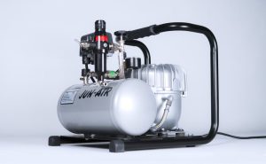
The Elveflow OB1 arrives configured with the channel count and pressure ranges you choose, driven from the Elveflow Smart Interface, with SDKs for Python, MATLAB, LabVIEW and C++ if you want to script it. Around it sits the fluidic line, and Elveflow supplies all of it. A pressure and vacuum source if you have no house air line, the reservoirs and their caps, the adapters and tubing. An MFS or BFS flow sensor to close the loop on flow, a MUX distribution valve to bring several precursors, a crosslinker or a wash down one line, and the chip at the far end. The OB1 drives the precursor and reports what it did; the chemistry and the curing are yours.
It drifts in pressure mode, and it holds in sensor mode, so the answer depends on which of the two you are running. In pressure mode you enter a pressure and the flow is whatever that pressure produces through your circuit, following Q = ΔP/R. As the precursor gels, R rises, and the flow falls even though the pressure is exactly where you left it. In sensor mode an Elveflow MFS or BFS sensor measures the flow and the Elveflow OB1 moves the pressure to match the value you asked for, holding a thickening precursor at a set flow rate through a long print. Pick pressure mode when the pressure is the physically meaningful quantity, and sensor mode when your geometry depends on the flow rate.
The Elveflow OB1 responds in about 10 ms, fast enough to make ink switching a structural tool. Published work alternating two ink channels with switching times down to 0.5 s produced fibre segments below 500 µm inside one continuous print. That 10 ms is the pressure at the controller; the flow at your nozzle settles afterwards, through the resistance and compliance of your tubing and chip, so short, stiff, narrow tubing gets you closer. A size change is the same operation, a new setpoint with no hardware to move. Where you need more materials than you have channels, or in a set order, an Elveflow MUX distribution valve switches between precursors on one line.
Count one channel per phase that has to flow at the same time as the others. A flow-focusing or coaxial geometry needs two, a core-shell with a carrier phase needs three, and a formulation whose proportions you set needs one per component. The Elveflow OB1 goes up to four independent channels in one instrument, each with its own setpoint and its own range, and it can be upgraded later if the geometry grows. Where the materials arrive in turn instead, one channel and an Elveflow MUX distribution valve carry several precursors down the same line. That screens a series of formulations on one chip at one setpoint, and keeps your channels for the phases that must run together. If you are unsure how your geometry maps onto channels, send us the design and we will go through it with you.
Yes, and it is one of the common ways the Elveflow OB1 is used in this field. You drive the aqueous precursor on one channel and the continuous phase on another. The ratio between those two setpoints, with your chip’s junction, sets the drop size, and the steadiness of both lines keeps the size distribution from spreading. Sweeping the ratio maps the dripping and jetting regimes in one session, with each point kept as a setpoint you can return to. An Elveflow MFS or BFS sensor closes the loop on either phase when a flow rate is the quantity you specify. Gelation stays your step: an ionic bath, a temperature change or a light source. For a turnkey spherical-bead setup Elveflow publishes a dedicated application pack, with the OB1 as the controller inside it. For core-shell drops, several compartments in one microgel or non-spherical particles, the same instrument drives the extra inlets.
The Elveflow OB1 comes in five ranges that together span −900 mbar to 8 bar, two of them combining vacuum with pressure. With an Elveflow MFS or BFS sensor closing the loop, the flow rates in reach run from 0.1 µL/min to 500 mL/min. The limit comes from the circuit: Q = ΔP/R, so the flow you get at a given pressure depends on tubing bore and length, nozzle diameter and the viscosity of your precursor. Choose the smallest range that covers your working pressures, because the stability and the minimum increment are both fractions of full scale.
It changes the resistance, not the way you work. A more viscous precursor means a higher R, so the same pressure gives a lower flow rate and you raise the setpoint to compensate. The Elveflow OB1 is offered up to 8 bar for that reason, and shorter, wider tubing is worth the trouble on a thick ink. If the viscosity climbs during the run, an Elveflow MFS or BFS sensor in the loop holds the flow rate as R rises. Where a precursor is too thick for the pressure available, our PSD syringe pump imposes the flow rate by displacement instead, and viscosity does not shift it in steady state. Send us the formulation and the viscosity you work at, and we will tell you which of the two routes holds up on your bench.
None of the instrument does. The Elveflow OB1 is a non-contact pump: it acts on the gas above the liquid, so your precursor stays inside its own path and the controller adds no dead volume. That path is your reservoir, the reservoir adapter, the tubing and your chip or nozzle. Elveflow tubing is PTFE, and each fluidic part lists its own wetted materials on its product page, so you can match your formulation and your solvents against them yourself. A flow sensor, when you use one, sits in that path too and lists its own wetted materials. Fewer parts in contact also means fewer places for a precursor to sit and start crosslinking.
Read it as a resistance problem, and the pressure tells you where it is. On the Elveflow OB1 in sensor mode, a rising pressure at a held flow rate says R is climbing, a partial blockage forming. In pressure mode the same event shows as a falling flow rate at a fixed pressure. To locate it, take the chip off and repeat: if the pressure needed drops back to its earlier value, the restriction is in the chip or nozzle, otherwise it is in the tubing, an adapter or a sensor channel. Crosslinked precursor at the nozzle, a partly cured plug from an earlier run and particles in a filler are the usual causes here. An Elveflow MPS pressure sensor with an MSR reader logs the pressure so you can see the rise starting instead of finding it afterwards, and a sequence can stop the run on a threshold.
Yes, and it is how most long runs are done. You build the pressure programme once in the Elveflow Smart Interface, give each stage its own duration, and the Elveflow OB1 works through it from the first drop to the last. Nobody has to sit at the panel, and the same file gives the same run next week, so a repeat batch compares with the first. Pressure and flow stream to CSV throughout, so you can see afterwards what the instrument actually did at every stage.
Yes, in both directions. The Elveflow OB1 has TTL lines in and out, at 0 or 5 V. It can start a sequence on a trigger from your motion controller, or fire a camera, a shutter or a UV source at a chosen step of its own sequence. The sequence is built once in the Elveflow Smart Interface and replayed, and pressure and flow stream to CSV while it runs, so each object comes with the settings that produced it. For tighter integration the SDKs drive the OB1 from Python, MATLAB, LabVIEW or C++, which is the usual route when the pressure has to follow a print path computed elsewhere.
That is the practical reason to drive a fabrication line by pressure. With the Elveflow OB1 the operating point is a number and a sequence you replay, held to 0.005% of full scale. The same file gives the same setpoints in another operator’s hands on another day, and the log shows what actually happened. The scatter left in your geometry then comes from the material and the chip. It also makes the method publishable: you report the value you set, with its range and its stability, and another lab has what it needs to reproduce your conditions.
It depends on the quantity you need to hold. The Elveflow OB1 pressure controller is the answer when the pressure is the meaningful quantity, and when you move between operating points during a run. It responds in about 10 ms, holds the pressure to 0.005% of full scale, and adds no moving part to the liquid. Ink switching, flow focusing, stop-flow cycles and fast size sweeps all sit here. Our PSD syringe pump takes the cases built the other way round, where you need a known delivered volume, or a flow rate that stays put as downstream resistance rises. The two coexist on the same bench. Tell us your precursor, your nozzle and what you need to keep constant, and we will settle it on your configuration.
Contact us through the form with your material system, the geometry you are making and the pressures or flow rates you work at. We will come back with an Elveflow OB1 configuration that fits, and answer setup questions before you buy.


 Job
Job Collaborations
 Customer
 Other
Other