Flow Control for Rheometry & Permeability
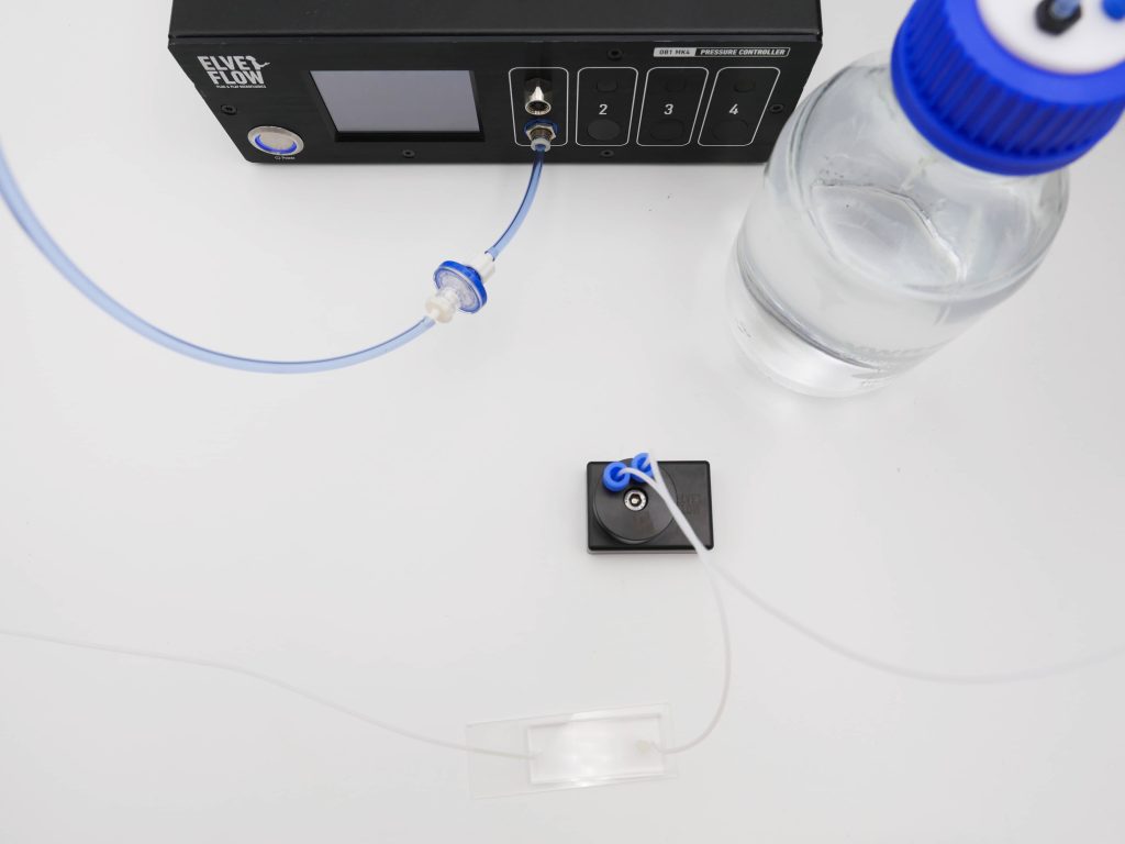
Each point you measure is taken at the pressure you set, or at a flow rate held with a flow sensor.A sequence steps the pressure and logs it throughout.
Held down to 0.005% of full scale by a piezo valve.
Each line carries its own pressure and range.
A saved sequence replays every setpoint.
The pressure drop across the capillary or chip is yours to set, anywhere from −900 mbar to 8 bar. Combine it with the flow rate you measure, and your model gives you the viscosity or the Darcy permeability.

-

Seongjin Park, Senior Engineer
Department of Physics, Syracuse University
We use Elveflow instrument in several projects and they are great to work with. The LabVIEW implementation was also very successful. I hope more people can get to know the OB1 system -

Dr. Pushparani Micheal Raj
Max Planck Institute of Quantum Optics, MAX IV Laboratory
I have extensively used Elveflow systems in the world's most brilliant X-ray source. Elveflow systems are precise, controlled and adaptive to many samples under adverse conditions. -

Dr. Hayden Taylor
University of California, Berkeley, United States
We are using the device extensively at the moment and I have been quite impressed by its capabilities -

Dr. Arne Lüken
Chemical Process Engineering at RWTH Aachen
The Elveflow OB1 enables us precise pressure and flow control and measurement in various microfluidic and lab scale projects from tissue engineering to membrane filtration analysis. -

Dr. Nelson BC Serre & Dr. Matyáš Fendrych
Cell Growth Lab, Department of Experimental Plant Biology, Charles University, Czech Republic
After an easy installation, we are now using the OB1 and flow sensors routinely and are very satisfied by both the flow stability and the software user-friendly interface.
Features & Benefits
How rheometry and permeability measurements are driven today
Getting a viscosity out of a capillary takes two numbers and a model. You push the sample through it at a known pressure drop, then measure the resulting flow rate with a flow sensor or an optical readout. The dimensions of the capillary turn that pair into a viscosity. Permeability works the same way, with Darcy’s law replacing the capillary model. So whatever happens to the pressure during the run ends up in the viscosity or the permeability you calculate.
A slow drift in pressure during a sweep shifts the whole flow curve. A small ripple turns into scatter between repeat points, which is easy to mistake for variability in the sample. And when the pressure overshoots after a step, the first points of that step are taken at the wrong pressure. The usual ways of driving the flow mostly differ in how well they avoid these problems.
Hydrostatic pressure. The simplest option is to raise the reservoir above the inlet, the way gravity capillary viscometers work. You need no power and no tuning, and the pressure is as steady as the liquid column that creates it. But nothing actually controls that pressure. The height of the column sets it, and no feedback corrects it during the run. To change it, you have to move the reservoir. As the liquid drains, the pressure also drops, which puts a slow drift on every point of a sweep.
A home-built pressure regulator. Some labs build a regulator themselves, from a proportional solenoid valve and a microcontroller. One published open-source design holds the pressure to about ±0.7 mbar on a single channel. Its authors also note that every regulator built this way has to be tuned individually, so two of them can hold the pressure differently. If another lab makes one to reproduce your conditions, part of the difference between your viscosity or permeability values and theirs can come from that tuning.
Proportional valve pressure control. Inside several commercial pressure controllers, the same kind of valve regulates the gas above the liquid. A coil pulls a plunger against a spring, and the current sets how far the valve opens, without any switching. But the plunger slides in a guide, and friction makes it move in small jumps when the correction is very fine. Around the setpoint, the controller keeps correcting back and forth, which can add fine scatter to the points of a sweep. It is also much slower to respond, and slower still with larger sample volumes, so each sweep step takes longer to settle.
Piezoelectric pressure control. Here the controller sets the pressure of the gas above the liquid, so nothing mechanical touches the sample. How well that pressure holds comes down to the valve. A valve that switches on and off tends to overshoot each new setpoint and then oscillate a little around it. That leaves a small periodic signal on every point of a sweep. A piezoelectric valve never switches, and since it deforms without any part sliding against another, it can make very small corrections smoothly. Ours holds the pressure down to 0.005% of full scale.
Every point of a flow curve starts from a pressure you choose
Pressure-driven flow follows Q = ΔP/R. You pick the pressure difference ΔP, and the resistance R of the line and the sample decides the flow rate Q you get. In a capillary, the pressure drop sets the shear stress at the wall and the flow rate gives the shear rate, so their ratio is the apparent viscosity. In a porous sample, the same two numbers give the Darcy permeability. On a shear-thinning sample, R also changes with the flow, and the flow rate has to be measured since the pressure alone can’t predict it.
Each pressure module covers one range. A capillary that barely resists the flow works with the 200 mbar range, and a narrow bore or a thick sample may need up to 8 bar. Within a range, the smallest pressure step is 0.006% of full scale, so you can space the points of a sweep as closely as you like. Since the controller only acts on the gas, it adds no dead volume and no wetted surface to the liquid path.
With a sensor, the flow rate holds when the resistance changes
When you control the pressure, the flow rate follows whatever resistance the circuit has. On a rheometry or permeability setup, that resistance rarely stays put. A suspension settles, a packed sample compacts under the flow, or the viscosity shifts with the temperature, which is yours to control. Without a sensor, the pressure stays at its setpoint and the flow drifts along with these changes. Add a flow sensor to the line and the controller corrects the pressure from the sensor’s reading, so the flow rate holds at your setpoint for the whole run.
Steady state before you record each point
When you change the setpoint, the controller responds in about 10 ms, whatever the sample volume. That figure is for the pressure at the controller, though. So each step of a sequence gets a dwell time, and you only take the data point once the flow has reached steady state.
That dwell saves you from redoing a sweep because its first points never settled. One sequence can also chain the pressure profiles of a creep and recovery test, a ramp across the shear rates and a sine at each frequency you want to probe.
Several conditions, each on its own line
The controller drives up to four channels, each with its own setpoint and pressure range. You can compare up to four conditions side by side, or bring two phases together at a pressure ratio you choose. One channel can also pressurise several reservoirs at once, so those samples run in parallel at the same pressure. If your samples come one after another, a distribution valve sends each of them through the same line in turn. They all go through one capillary, and since nothing is taken apart between samples, the geometry is the same for all of them.
The sweep runs on its own and keeps a log
You write the sequence once in our software, with a setpoint and a duration for each step. The controller then runs through it on its own, overnight if needed. Meanwhile the software logs the pressure, plus the flow if a sensor is connected, so you can later match any point of your sweep to the pressure at that moment. TTL inputs and outputs also link the sequence to a camera or an acquisition card. And if the pressure has to follow a value computed elsewhere, you can script the controller in Python, MATLAB, LabVIEW or C++ through the SDKs.
Will another lab reproduce your conditions?
On the same controller, repeating a measurement is easy, because a saved sequence replays the same pressures step by step. For someone else to reproduce it, whether in your lab or another, they also need the range and the stability those pressures were held to. With that on record, the pressure adds less scatter to your viscosity or permeability values, and most of what’s left comes from the sample, the geometry and the temperature.
Application
Semiflexible rod suspensions, shear viscosity
Salipante and colleagues wanted to follow how semidilute suspensions of fd bacteriophage thin under shear, up to shear rates that rotational rheometry rarely reaches [Macromolecules, 2025, 1]. Our pressure controller held the pressure drop across their capillaries. On less than a millilitre of sample, they covered nearly six decades of shear rate, and the curves didn’t depend on the size of the capillary. Repeat runs gave the same viscosity, a sign that the rods hadn’t broken under shear.
Effective permeability of etched pillar arrays
How much do the top and bottom walls of a channel slow the flow through a pillar array? Hulikal Chakrapani and colleagues tested four pillar arrays with different amounts of open space, while our controller maintained the pressure [Soft Matter, 2023, 2]. A Darcy fit across the pressure steps gave effective permeabilities from 1.23 to 5.06 µm² as porosity went up, with water and hexadecane agreeing within error. The chips resisted the flow only 6 to 25 times more than the same channel without pillars, so the authors conclude the walls can’t be ignored, especially at high porosity.
Breast tumour spheroids, stiffness and relaxation
To compare malignant MDA-MB-231 and non-tumorigenic MCF-10A spheroids while imaging them, Suh and colleagues built a microfluidic rheometer [Lab on a Chip, 2025, 3]. Our pressure controller drove the pressure in the chamber above a soft piston through static and cyclic profiles, and a gel under each spheroid acted as the force sensor. The malignant spheroids turned out softer, with a corrected Young’s modulus of 396.8 ± 60.1 Pa against 903.0 ± 111.9 Pa. Under square-wave loading they also relaxed more slowly, with half relaxation times of 8.7 ± 1.1 s against 3.1 ± 0.5 s.
[1] Salipante PF, Kuei S, Murphy RP, Fagan JA, Sims CM, Weigandt KM, Hudson SD. Rheology and Microstructural Behavior of Semidilute Suspensions of Semiflexible Rods across Five Decades of Shear Rate. Macromolecules. 2025;58(5):2389-2400. doi:10.1021/acs.macromol.4c02675
[2] Hulikal Chakrapani T, Bazyar H, Lammertink RGH, Luding S, den Otter WK. The permeability of pillar arrays in microfluidic devices: an application of Brinkman’s theory towards wall friction. Soft Matter. 2023;19(3):436-450. doi:10.1039/d2sm01261h
[3] Suh YJ, Liu M, Zhu B, Pandey M, Cheung BCH, Kim J, Bouklas N, Roh C, Segall JE, Hui CY, Wu M. A microfluidic rheometer for tumor mechanics and invasion studies. Lab on a Chip. 2025;25(22):6018-6032. doi:10.1039/d5lc00504c
| OB1 MK4 | |||||
|---|---|---|---|---|---|
| PNEUMATIC SPECIFICATION | |||||
| Channel pressure range | 0 to 200 mbar(1) (0 to 2.9 psi) |
0 to 2,000 mbar(1) (0 to 29 psi) |
0 to 8,000 mbar(1) (0 to 116 psi) |
-900 to 1,000 mbar(1) (-13 to 14.5 psi) |
-900 to 6,000 mbar(1) (-13 to 87 psi) |
| Pressure stability(2) | 0.015 % FS(1) 0 µbar (0.0004 psi) |
0.005 % FS(1) 100 µbar (0.0014 psi) |
0.006 % FS(1) 500 µbar (0.007 psi) |
-900 to 500 mbar | -900 to 2,000 mbar |
| 0.005 % FS(1) 100 µbar (0.0014 psi) |
0.005 % FS(1) 350 µbar (0.005 psi) |
||||
| 500 to 1,000 mbar | 2,000 to 6,000 mbar | ||||
| 0.007 % FS(1) 150 µbar (0.0021 psi) |
0.007 % FS(1) 525 µbar (0.0076 psi) |
||||
| Response time(3) | Down to 10 ms | ||||
| Setting time(4) | Down to 50 ms | ||||
| Minimum pressure increment | 0.006 % FS(1) 12 µbar (0.00017psi) |
0.006 % FS(1) 120 µbar (0.0017 psi) |
0.006 % FS(1) 480 µbar (0.007 psi) |
0.0064 % FS(1) 120 µbar (0.0017 psi) |
0.0064 % FS(1) 420 µbar (0.006 psi) |
| Pressure supply | 1.5 bar (or Max pressure + 0.5 bar) to 10 bar Non corrosive, non explosive, dry and oil-free gases, e.g. air, argon, N2, CO2, … |
||||
| Input vacuum(5) | / / |
Any value from -0.7 to -1 bar Compatible with vacuum pump or vacuum line |
|||
| Input pneumatic connector | 6 mm push-in | ||||
| Output pneumatic connector | 4 mm push-in | ||||
| Liquid compatibility | Non contact pump Any aqueous, oil, or biological sample solution. |
||||
| FLOW CONTROL | |||||
| Flow sensor compatibility | Compatible with the whole MFS and BFS range Monitoring and feedback loop flow control available | ||||
| Flow sensor compatibility | From 0,1 µL/min to 500 mL/min (indicative, please refer to the MFS and BFS series) | ||||
| Flow sensor compatibility | Non-contact pump Any aqueous, oil, or biological sample solution. | ||||
| CONTROL & MONITORING | |||||
| Software control | Elveflow Smart Interface – Windows 10, 11, both 32 and 64 bit versions supported | ||||
| Software Development Kit | Libraries available: Matlab, Python, LabView, C++ | ||||
| Flow sensor compatibility | Non-contact pump Any aqueous, oil, or biological sample solution. – Windows 10, 11, both 32 & 64 bit versions supported Serial/UART communication protocol on request | ||||
| Data management | Possibility to log and extract data (CSV), channel and sensor detailed information using ESI | ||||
| Input profiles | Possibility to load profiles: ramp, sine, triangle, square, or custom | ||||
| Automation | Generate step-by-step sequences using the ESI built-in sequence management Log and export custom configurations (CSV) | ||||
| Screen | LCD screen showing pressure and sensor flow rate in real time | ||||
| ELECTRICAL SPECIFICATIONS | |||||
| Voltage | 24V | ||||
| Typical power | 12W | ||||
| Power connection | DC power connector, Plug, 3A, 2.1mm, 12mm | ||||
| Interface | USB Type B | ||||
| Communication type | Serial | ||||
| Sensor connection | M8 4-pins, one connector per channel | ||||
| Compatibilit | Elveflow sensors: MFS, BFS, MPS, MFP, MBD Custom sensors: 5 to 24V supply voltage, 0 to 10V readout voltage | ||||
| Triggers | Input and Output TTL signal 0V or 5V | ||||
| Supply Voltage Range (V) | 100 to 240 VAC | ||||
| Supply AC Frequency (Hz) | 50 to 60 Hz | ||||
| Maximum Output Current (A) | 1.67 A | ||||
| Maximum Output Power (W) | 40 W | ||||
| MECHANICAL SPECIFICATIONS | |||||
| Dimensions (length x width x height) | 240 x 223 x 83 mm | ||||
| Weight | 1.4 kg to 2.9 kg | ||||
(1) Max pressure value might vary by +/- 2.5% (2) Pressure stability (standard deviation) measured over the full pressure range with an external high accuracy pressure sensor (Druck DPI150) (3) Time required to reach 5% of the setting point. Depending on your computer’s operating system (4) Time required to reach 95% of the set point. Volume dependent – Measurement was done on 12 mL reservoir for a set point from 0 to 200 mbar (5) A vacuum source is mandatory for calibration and use of dual channels even if the channels are to be used in pressure only.
Frequently Asked Questions
Yes, the Elveflow OB1 handles the pressure side. It pressurises the gas above each reservoir, so you choose the pressure difference across the capillary or chip and the controller holds it. Add an Elveflow flow sensor to the line and you can also set the flow rate itself, while the controller corrects the pressure to reach it. Your model then combines the two with the dimensions of the geometry to give a viscosity or a Darcy permeability. If the tubing upstream adds noticeable resistance, an Elveflow MPS pressure sensor at the inlet measures the pressure that actually reaches the geometry.
The Elveflow OB1 comes configured for the number of channels and the pressure ranges you need, and our software and the SDKs are included. We also supply the rest of the fluidic line, from the gas and vacuum source to the reservoirs and caps, the adapters, the tubing, the flow sensors and the chip. If trapped gas could spoil a reading, a bubble remover can go into the line. The sample stays on your side, together with its temperature control and the detector that reads the response.
The Elveflow OB1 comes in five pressure ranges, up to 8 bar, and two of them go down to −900 mbar of vacuum. With a flow sensor closing the loop, you can hold flow rates from 0.1 µL/min to 500 mL/min, depending on the sensor. How much flow a given pressure produces depends on the tubing, the geometry and the viscosity of your sample, so in practice the circuit sets the limit. Pick the lowest range that still covers your working pressures, since the stability and the smallest pressure step are both a fraction of full scale.
In pressure mode, the Elveflow OB1 holds the pressure you entered, and the flow rate follows the circuit. If the resistance goes up, the flow drops while the pressure stays put. Add an Elveflow MFS or BFS flow sensor and the controller switches to sensor mode, adjusting the pressure until the measured flow matches your setpoint. The flow rate then holds even when a suspension settles, a sample compacts or the liquid warms up. For capillary rheometry and Darcy measurements, pressure mode is usually the natural choice, since your model starts from the pressure drop.
No part of the Elveflow OB1 touches your sample, since the controller only pressurises the gas above it. On its way, the sample meets the reservoir and its adapter, the tubing, any flow sensor or valve in the line, and the capillary or chip you measure in. We give you the wetted materials of every part we propose, so you can check them against your sample.
A clog shows up as a rising resistance. In sensor mode, the Elveflow OB1 raises the pressure to hold the flow rate at your setpoint as the blockage forms. In pressure mode, the pressure doesn’t move and you see the flow rate fall. To find where it is, take the capillary or chip out and repeat the step. If the pressure goes back to what it was, the blockage was in that part. If not, check the tubing, an adapter or the sensor channel. The usual culprits are aggregates in a suspension or fine particles shed by a packed sample.
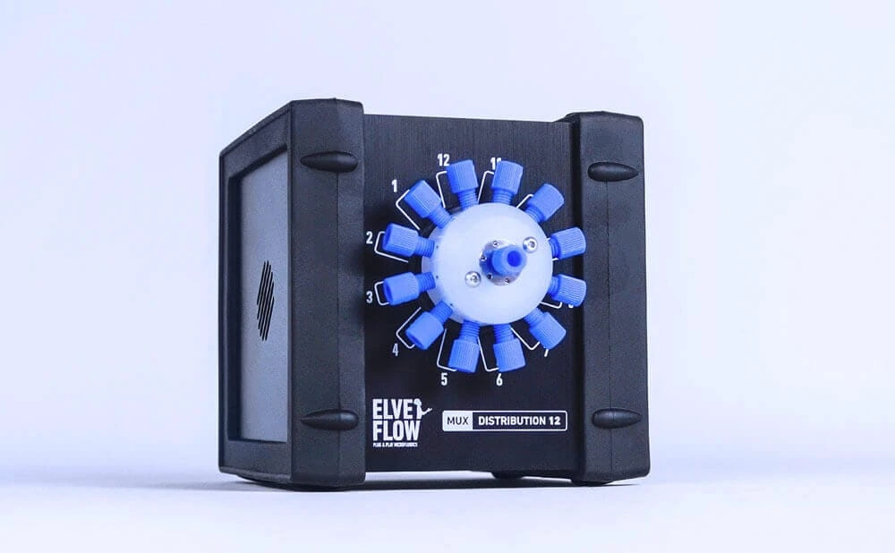
Yes, you can. The Elveflow OB1 drives up to four channels, each with its own pressure and range. You can compare up to four conditions in parallel, or bring two phases together at a pressure ratio you choose. One channel can also pressurise several reservoirs at once, so all those samples run at the same pressure. To switch these lines on and off, or to route four inputs to four outputs, add an Elveflow MUX Flow Switch Matrix or a MUX Cross Chip. If your samples come one after another, an Elveflow MUX Distribution valve sends each one through the same capillary at the same setpoint, which takes geometry out of the comparison.
Yes, and for a long sweep it’s really the way to go. You build the sequence once in the Elveflow Smart Interface (ESI), with a setpoint and a duration for each step. The Elveflow OB1 then runs through it with nobody at the panel. Meanwhile the software logs the pressure to a CSV file, plus the flow when a flow sensor is connected. From that log you can check that the flow had settled at each pressure step. Run the same file a month later and you get the same sequence of pressures, which keeps two measurement campaigns comparable.
It works both ways. The Elveflow OB1 has TTL inputs and outputs at 0 or 5 V. An external trigger can start a sequence, and the sequence can fire your camera or detector at the step you choose. Each pressure step then lines up in time with the frame that records its response. And if the pressure has to follow a value computed from the measurement itself, you can drive the controller in Python, MATLAB, LabVIEW or C++ through the SDKs.
It works best as a complement. Your bench rheometer stays the reference for what it already measures, and a microfluidic setup covers what it leaves open. In that setup, the Elveflow OB1 applies the pressure, while the measurement itself comes from the capillary or chip and your readout. A capillary needs less than a millilitre of sample, which helps when the sample is scarce. Driven by pressure, it can also reach wall shear rates beyond the usual limit of rotational rheometry. And you can measure inline in a microfluidic process, or run several lines in parallel.
You build it term by term, as for any measurement chain. The Elveflow OB1 handles the pressure term and keeps it small. The pressure is a number you entered, held down to 0.005% of full scale and logged for the whole run. The other terms usually dominate, and they come from the geometry, the flow measurement, the model and the temperature. Send us the measurement you have in mind, and we’ll go through the pressure contribution to its uncertainty with you.
Tell us through the contact form what you measure, in which geometry, how much sample you have and the pressure or flow range you expect. We’ll size an Elveflow OB1 for it, tell you which pressure range to pick and answer your setup questions before you buy.



 Job
 Collaborations
 Customer
 Other